Get started with mascaret#
The mascaret module is a linear oscillation code fully written in Python and dedicated to computing eigenfunctions of stellar modes of oscillations considering an equatorial-channel approximation of rotation. The following tutorial is aimed at introducing the main functionalities of the module.
import mascaret as em
import matplotlib.pyplot as plt
em.__version__
'0.2'
After importing the module, we can start by setting some parameters for the mode exploration we will carry out.
# Solver to use, that will be passed to scipy.integrate.solve_ivp
em.solver_kwargs["method"] = "RK23" #default solver is RK45
em.solver_kwargs["max_step"] = 1e-3
# Number of nodes to use for the parallelised step
nodes = 8
# Grid search method, frequency interval to explore, and number of
# grid points to consider
method = "inverse"
omega_0, omega_1 = 20, 30 #(muHz)
n_grid = 300
# Angular degree and azimuthal number of the modes to look for
l_m = {1:[1]}
The module includes an example stellar profile of a 1 \(\rm M_\odot\) star that was computed with MESA.
model = em.load_example_profile ()
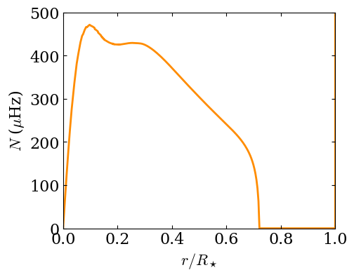
In the first steps of this tutorial, we will compute the properties of dipolar (\(\ell=1\)) gravity modes (g modes) in the example stellar profile. The Brunt-Väisälä frequency, \(N\), is the key physical quantity to consider when dealing with these modes, which will be propagative only when \(N>0\) (radiative stratified regions) and evanescent otherwise (convective regions).
fig, ax = plt.subplots (1, 1, figsize=(5,4))

ax.plot (model.x, model.N,
         lw=2, color="darkorange")
ax.set_xlabel (r"$r/R_\star$")
ax.set_ylabel (r"$N$ ($\mu$Hz)")
ax.set_xlim (0, 1)
ax.set_ylim (0, 500)
(0.0, 500.0)
A case without rotation#
We start by considering a case without rotation.
rot_solar_rate = 0
Depending on the chosen search method (simple or double shooting), it is possible to define a \(\Delta (\omega)\) function (with \(\omega\) the wave frequency) for which the eigenmodes of the problem will correspond to \(\Delta (\omega) = 0\). The frequency grid is thus scanned to search for occurrences where \(\Delta (\omega)\) changes sign, then the eigenfrequencies and eigenfunctions are refined by performing a dichotomy search around the found intervals.
results = em.mode_search (model,
                        l_m,
                        omega_0=omega_0,
                        omega_1=omega_1,
                        n_grid=n_grid,
                        rot_solar_rate=rot_solar_rate,
                        method=method,
                        parallelise=True,
                        nodes=nodes,
                        double_shooting=True,
                        output_dir="quickstart",
                        start_full_span="stitch")
Looking for l=1, m=1 modes.
Iterating on grid chunks.
9it [00:04, 1.96it/s]
11 zeros found
100%|███████████████████████████████████████████████████████████████████████████████████████████████████████████████████████████| 11/11 [00:09<00:00, 1.11it/s]
results
| n | n_g | n_p | l | m | nu | delta | transmission | rot_solar_rate |
|---|---|---|---|---|---|---|---|---|
| int32 | int32 | int32 | int32 | int32 | float32 | float32 | float32 | float32 |
| -33 | -33 | 0 | 1 | 1 | 20.371603 | 0.0 | -0.12487564 | 0.0 |
| -32 | -32 | 0 | 1 | 1 | 20.995756 | 0.0 | -0.13381477 | 0.0 |
| -31 | -31 | 0 | 1 | 1 | 21.66339 | 0.0 | -0.14416665 | 0.0 |
| -30 | -30 | 0 | 1 | 1 | 22.372078 | 0.0 | -0.15531035 | 0.0 |
| -29 | -29 | 0 | 1 | 1 | 23.126274 | 0.0 | -0.16792531 | 0.0 |
| -28 | -28 | 0 | 1 | 1 | 23.937809 | 0.0 | -0.181721 | 0.0 |
| -27 | -27 | 0 | 1 | 1 | 24.80276 | 0.0 | -0.19798696 | 0.0 |
| -26 | -26 | 0 | 1 | 1 | 25.736795 | 0.0 | -0.21623734 | 0.0 |
| -25 | -25 | 0 | 1 | 1 | 26.738888 | 0.0 | -0.23738325 | 0.0 |
| -24 | -24 | 0 | 1 | 1 | 27.823713 | 0.0 | -0.26373035 | 0.0 |
| -23 | -23 | 0 | 1 | 1 | 28.997177 | 0.0 | -0.2918132 | 0.0 |
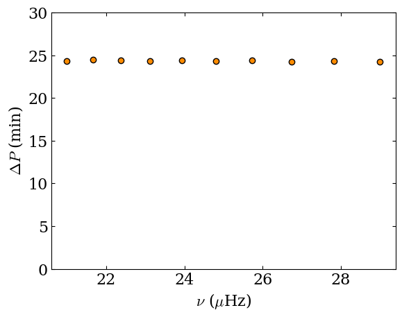
An important property of the gravity modes we are considering here is that their period spacing is asymptotically constant (\(|n|\gg1\)).
delta_p = - np.diff (1e6/(results["nu"]*60))

fig, ax = plt.subplots (1, 1)

ax.scatter (results["nu"][1:], delta_p, marker="o",
            color="darkorange", edgecolor="black")

ax.set_xlabel (r"$\nu$ ($\mu$Hz)")
ax.set_ylabel (r"$\Delta P$ (min)")

ax.set_ylim (0, 30)
(0.0, 30.0)
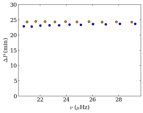
Including rotation#
Let us now consider the rotating case. Note that, in mascaret, the
stellar rotation rate has to be provided in unity of solar rotation
frequency (which is set to 4.14e-7 Hz, and can be accessed through
the mascaret.solar_rotation_frequency global variable). It is
possible to set a uniform rotation rate by passing rot_solar_rate as
a float; radial rotation profile are also accepted, in this case, the
variable has to be provided as an array.
rot_solar_rate = 50
results_rot = em.mode_search (model,
                            l_m,
                            omega_0=omega_0,
                            omega_1=omega_1,
                            n_grid=n_grid,
                            rot_solar_rate=rot_solar_rate,
                            method=method,
                            parallelise=True,
                            nodes=nodes,
                            double_shooting=True,
                            output_dir="quickstart",
                            start_full_span="stitch")
Looking for l=1, m=1 modes.
Iterating on grid chunks.
9it [00:07, 1.27it/s]
12 zeros found
100%|███████████████████████████████████████████████████████████████████████████████████████████████████████████████████████████| 12/12 [00:11<00:00, 1.07it/s]
results_rot
| n | n_g | n_p | l | m | nu | delta | transmission | rot_solar_rate |
|---|---|---|---|---|---|---|---|---|
| int32 | int32 | int32 | int32 | int32 | float32 | float32 | float32 | float32 |
| -34 | -34 | 0 | 1 | 1 | 20.181133 | 0.0 | -0.17386039 | 50.0 |
| -33 | -33 | 0 | 1 | 1 | 20.754906 | 0.0 | -0.18290704 | 50.0 |
| -32 | -32 | 0 | 1 | 1 | 21.36104 | 0.0 | -0.19318701 | 50.0 |
| -31 | -31 | 0 | 1 | 1 | 22.011572 | 0.0 | -0.2050534 | 50.0 |
| -30 | -30 | 0 | 1 | 1 | 22.706648 | 0.0 | -0.21858346 | 50.0 |
| -29 | -29 | 0 | 1 | 1 | 23.4481 | 0.0 | -0.23327672 | 50.0 |
| -28 | -28 | 0 | 1 | 1 | 24.246815 | 0.0 | -0.24978416 | 50.0 |
| -27 | -27 | 0 | 1 | 1 | 25.100496 | 0.0 | -0.27011144 | 50.0 |
| -26 | -26 | 0 | 1 | 1 | 26.025555 | 0.0 | -0.2911211 | 50.0 |
| -25 | -25 | 0 | 1 | 1 | 27.017998 | 0.0 | -0.31664476 | 50.0 |
| -24 | -24 | 0 | 1 | 1 | 28.09541 | 0.0 | -0.34629923 | 50.0 |
| -23 | -23 | 0 | 1 | 1 | 29.261377 | 0.0 | -0.38139284 | 50.0 |
delta_p_rot = - np.diff (1e6/(results_rot["nu"]*60))

fig, ax = plt.subplots (1, 1)

ax.scatter (results["nu"][1:], delta_p, marker="o",
            color="darkorange", edgecolor="black")
ax.scatter (results_rot["nu"][1:], delta_p_rot, marker="o",
            color="blue", edgecolor="black")

ax.set_xlabel (r"$\nu$ ($\mu$Hz)")
ax.set_ylabel (r"$\Delta P$ (min)")

ax.set_ylim (0, 30)
(0.0, 30.0)
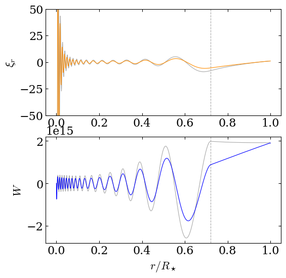
Comparing the eigenfunctions#
n = results["n"][0]
mode = em.load_eigenfunction ("quickstart/nabs{}_n{}_l1_m1_0_solar_rot.h5".format (str (np.abs (n)).zfill (4),
                                                                                     str (n).zfill (4)))
mode_rot = em.load_eigenfunction ("quickstart/nabs{}_n{}_l1_m1_{}_solar_rot.h5".format (str (np.abs (n)).zfill (4),
                                                                                     str (n).zfill (4),
                                                                                         rot_solar_rate))
fig = em.plot_eigenfunction (mode["x"],
                             mode["xi_r"]/model.R,
                             mode["W"],
                             axs=None, model=model, omega=None,
                             rot_solar_rate=None,
                             c1="darkgrey", c2="darkgrey")
axs = fig.get_axes ()
_ = em.plot_eigenfunction (mode_rot["x"],
                           mode_rot["xi_r"]/model.R,
                           mode_rot["W"],
                           axs=axs, model=None, omega=None,
                           rot_solar_rate=None,
                           c1="darkorange", c2="blue")

axs[0].set_ylim (-50, 50)
(-50.0, 50.0)
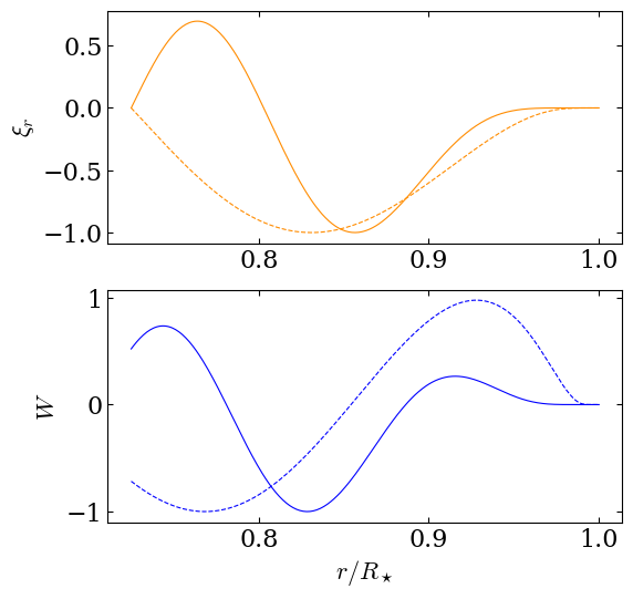
Eigenfunction of a truncated shell#
It is also possible to compute the eigenfunction considering an inner boundary located upper than the centre. We can for example explore the behaviour of the isolated convective envelope in order to take a look at the properties of pure inertial modes. For simplicity, we choose to force the buoyancy of the medium to remain neutral (\(N^2 = 0\)).
model = em.load_example_profile (convective_neutral=False,
                                 remove_atmosphere=True)
rot_solar_rate = 1
# Considering only the convective envelope
x_span = (model.x[model.index2+1], 1)
omega_0, omega_1 = 0.02, 0.1
xf = 0.85
method = "linear"
results_truncated = em.mode_search (model,
                                    l_m,
                                    omega_0=omega_0,
                                    omega_1=omega_1,
                                    n_grid=n_grid,
                                    rot_solar_rate=rot_solar_rate,
                                    method=method,
                                    parallelise=True,
                                    nodes=nodes,
                                    double_shooting=True,
                                    output_dir="quickstart",
                                    start_full_span="stitch",
                                    x_span=x_span,
                                    xf=xf)
Looking for l=1, m=1 modes.
Iterating on grid chunks.
9it [00:04, 1.95it/s]
2 zeros found
100%|█████████████████████████████████████████████████████████████████████████████████████████████████████████████████████████████| 2/2 [00:01<00:00, 1.47it/s]
results_truncated
| n | n_g | n_p | l | m | nu | delta | transmission | rot_solar_rate |
|---|---|---|---|---|---|---|---|---|
| int32 | int32 | int32 | int32 | int32 | float32 | float32 | float32 | float32 |
| -3 | -3 | 0 | 1 | 1 | 0.027354332 | 0.0 | inf | 1.0 |
| -2 | -2 | 0 | 1 | 1 | 0.0662436 | 0.0 | -inf | 1.0 |
filename_1 = "quickstart/nabs0003_n-003_l1_m1_{}_solar_rot.h5".format (rot_solar_rate)
filename_2 = "quickstart/nabs0002_n-002_l1_m1_{}_solar_rot.h5".format (rot_solar_rate)
mode_truncated_1 = em.load_eigenfunction (filename_1)
mode_truncated_2 = em.load_eigenfunction (filename_2)

fig = em.plot_eigenfunction (mode_truncated_1["x"],
                           mode_truncated_1["xi_r"]/np.abs (mode_truncated_1["xi_r"]).max(),
                           mode_truncated_1["W"]/np.abs (mode_truncated_1["W"]).max(),
                           model=None, omega=None,
                           rot_solar_rate=None,
                           c1="darkorange", c2="blue")
axs = fig.get_axes ()
_ = em.plot_eigenfunction (mode_truncated_2["x"],
                           mode_truncated_2["xi_r"]/np.abs (mode_truncated_2["xi_r"]).max(),
                           mode_truncated_2["W"]/np.abs (mode_truncated_2["W"]).max(),
                           axs=axs,
                           model=None, omega=None,
                           rot_solar_rate=None,
                           c1="darkorange", c2="blue", ls="--")